

Example: hourly chilled-water temperature
168 observations: one temperature reading each hour for seven consecutive days.
Download the example data (CSV)This is the same example used in Help. Import the CSV to follow the steps, or use Open example in a practice copy in Help to prefill the inputs.
1. Create the workspace
In the sidebar, open Basic Statistics and choose Autocorrelation. Create an analysis, name it, select New blank worksheet, then choose Create analysis.
2. Import the example data
Download the CSV above and import it into the worksheet. Choose Comma as the delimiter, Dot as the decimal separator and First row contains column names.
3. Assign the ordered series
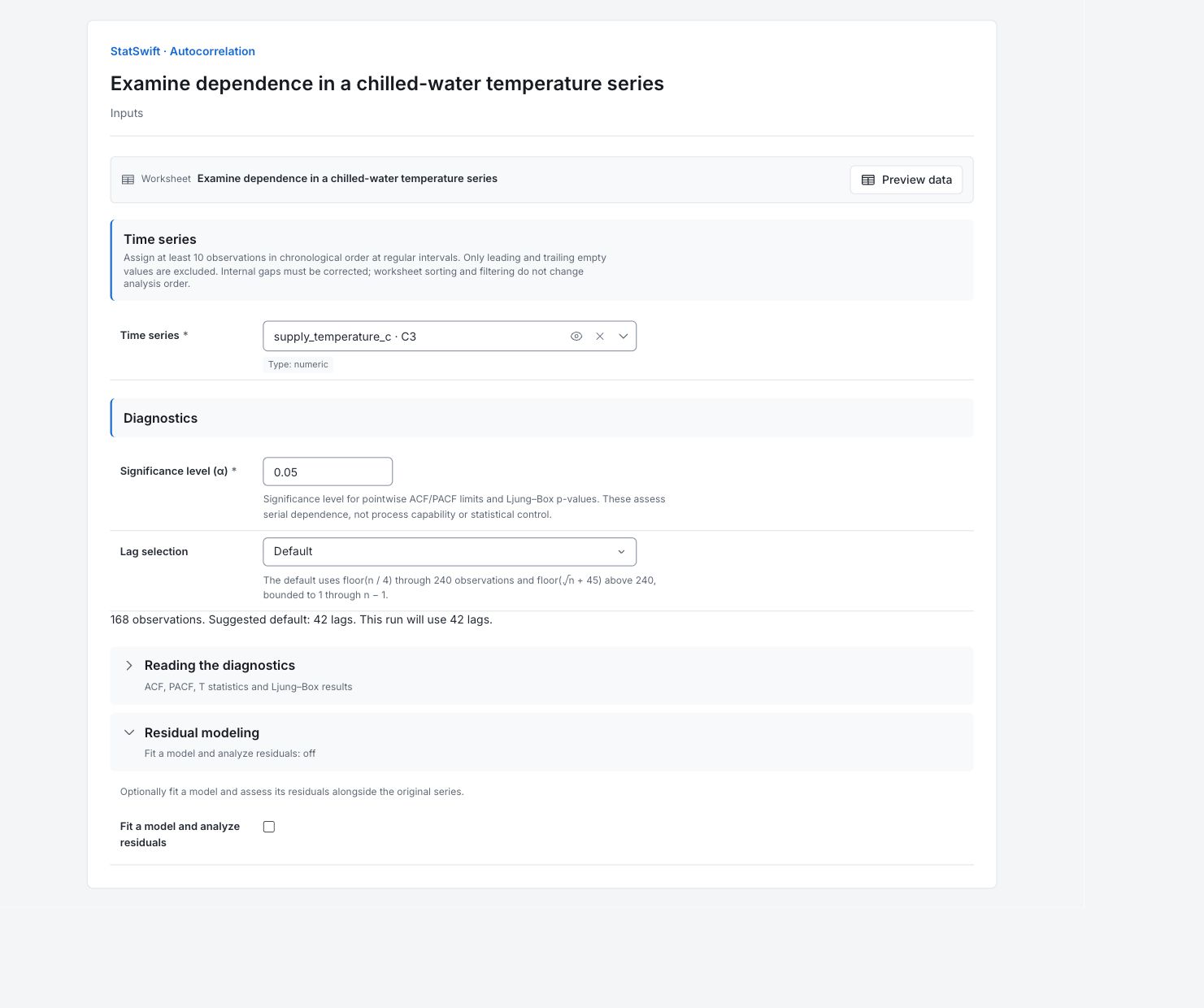
On Inputs, assign supply_temperature_c to Time series. Keep the 168 hourly readings in their recorded order. Do not remove internal gaps or assume worksheet sorting changes the analysis order.
4. Set the diagnostics
Enter 0.05 in Significance level (α). Choose Default for Lag selection; the status should show 42 lags for 168 observations. Open Residual modeling and leave Fit a model and analyze residuals unchecked.
5. Run analysis
Choose Run analysis, then open Results.
6. Interpret results
Read the lag axis
The 168 readings were collected hourly for seven days. Lag 1 compares neighboring hours; lag 24 compares readings one day apart. Correlations measure linear association, not a temperature difference.
Look for persistence and recurrence
ACF at lag 1 is about 0.91 and at lag 24 about 0.74. Both cross their displayed significance bounds. Temperatures tend to stay related over neighboring hours, with a recurring association a day apart. Review daily operating records; the plot does not identify a physical cause.

Series ACF View full-size chart (opens in a new tab) Read the partial correlations
At lag 2, ACF is about +0.77, while PACF is about −0.34 after accounting for lag 1. The raw two-hour association and the additional association after adjustment can differ in sign. Compare PACF with its pointwise bounds; this run fits no time-series model.

Series PACF View full-size chart (opens in a new tab) Read the combined test
Through lag 42, Ljung–Box Q is 2,246.90. Its extremely small p-value displays as 0 because of numerical precision, not because the probability is exactly zero. There is strong evidence of serial dependence.
Use the dependence in later work
Keep the hourly sequence and account for dependence in the next analysis. Counting all 168 readings as independent can overstate the available evidence. These diagnostics do not establish process control or capability.
More details: read each result section
Complete result tables use six significant digits, as in Help.
Series autocorrelation diagnostics
Effective observations is 168 and Final displayed / tested lag is 42. Alpha is 0.05 and Lag selection is Default. Calculation version identifies the diagnostic conventions. Ljung–Box Q and its p-value accumulate evidence through the final lag; read a displayed zero as a numerical reporting limit.
| Statistic | Value |
|---|---|
| Calculation version | 2 |
| Series | Ordered measurements |
| Effective observations | 168 |
| Alpha | 0.05 |
| Lag selection | Default (sample-size guidance) |
| Requested lags | Default |
| Final displayed / tested lag | 42 |
| Ljung–Box Q | 2246.9 |
| Ljung–Box DF | 42 |
| Ljung–Box p-value | 0 |
| Interpretation | Evidence of autocorrelation in the series through lag 42 (α = 0.05). |
Series correlations and cumulative Ljung–Box
Lag is separation in hours. ACF is correlation with that earlier value; PACF adjusts for intervening lags. ACF T is ACF divided by its standard error and tests one lag. LBQ, LBQ DF and LBQ p-value give the cumulative Ljung–Box test through each lag. All 42 rows are shown; later lags use fewer paired observations.
ACF T tests an individual lag. LBQ and its p-value combine lags 1 through the row’s lag.
| Lag | ACF | PACF | ACF T | LBQ | LBQ DF | LBQ p-value |
|---|---|---|---|---|---|---|
| 1 | 0.909726 | 0.909726 | 11.7914 | 141.535 | 1 | 1.22919e-32 |
| 2 | 0.769726 | -0.335709 | 6.12268 | 243.469 | 2 | 1.35295e-53 |
| 3 | 0.590476 | -0.257812 | 3.90555 | 303.82 | 3 | 1.48278e-65 |
| 4 | 0.392682 | -0.153431 | 2.3894 | 330.673 | 4 | 2.60783e-70 |
| 5 | 0.191901 | -0.112736 | 1.12992 | 337.125 | 5 | 1.03399e-70 |
| 6 | -0.0126268 | -0.192623 | -0.0737881 | 337.153 | 6 | 8.82606e-70 |
| 7 | -0.218903 | -0.237349 | -1.27918 | 345.654 | 7 | 1.04946e-70 |
| 8 | -0.404073 | -0.1235 | -2.33857 | 374.798 | 8 | 4.57796e-76 |
| 9 | -0.564829 | -0.172807 | -3.16745 | 432.104 | 9 | 1.91524e-87 |
| 10 | -0.692961 | -0.192586 | -3.67284 | 518.904 | 10 | 4.02031e-105 |
| 11 | -0.774349 | -0.13218 | -3.8097 | 627.98 | 11 | 1.44312e-127 |
| 12 | -0.797445 | -0.048621 | -3.62281 | 744.402 | 12 | 1.36661e-151 |
| 13 | -0.767302 | -0.0875804 | -3.24179 | 852.885 | 13 | 6.44296e-174 |
| 14 | -0.680068 | -0.0193745 | -2.70878 | 938.656 | 14 | 2.24161e-191 |
| 15 | -0.55157 | -0.0449476 | -2.10687 | 995.445 | 15 | 1.27574e-202 |
| 16 | -0.379982 | 0.0736759 | -1.41455 | 1022.57 | 16 | 1.64022e-207 |
| 17 | -0.181078 | 0.0576671 | -0.666207 | 1028.78 | 17 | 6.27864e-208 |
| 18 | 0.0264676 | 0.0296684 | 0.0971211 | 1028.91 | 18 | 4.64621e-207 |
| 19 | 0.2278 | 0.0428979 | 0.835849 | 1038.86 | 19 | 2.67704e-208 |
| 20 | 0.401449 | -0.027718 | 1.46692 | 1069.96 | 20 | 4.61875e-214 |
| 21 | 0.55164 | 0.0939007 | 1.99039 | 1129.08 | 21 | 8.27472e-226 |
| 22 | 0.664155 | 0.0343112 | 2.34177 | 1215.37 | 22 | 2.34917e-243 |
| 23 | 0.723244 | -0.0486439 | 2.47074 | 1318.39 | 23 | 1.75938e-264 |
| 24 | 0.736318 | 0.0384459 | 2.4287 | 1425.92 | 24 | 1.42531e-286 |
| 25 | 0.695007 | -0.0204701 | 2.21596 | 1522.4 | 25 | 2.65207e-306 |
| 26 | 0.60346 | -0.039452 | 1.87018 | 1595.64 | 26 | 0 |
| 27 | 0.482056 | 0.0689746 | 1.46378 | 1642.71 | 27 | 0 |
| 28 | 0.337829 | 0.0875217 | 1.01299 | 1665.99 | 28 | 0 |
| 29 | 0.178397 | 0.0782933 | 0.531689 | 1672.53 | 29 | 0 |
| 30 | 0.0149729 | 0.0729778 | 0.0445501 | 1672.58 | 30 | 0 |
| 31 | -0.166442 | -0.110348 | -0.495222 | 1678.35 | 31 | 0 |
| 32 | -0.348901 | -0.084198 | -1.03659 | 1703.91 | 32 | 0 |
| 33 | -0.505749 | -0.0176767 | -1.49306 | 1758.03 | 33 | 0 |
| 34 | -0.60323 | 0.185411 | -1.75767 | 1835.58 | 34 | 0 |
| 35 | -0.654539 | -0.0127267 | -1.87304 | 1927.58 | 35 | 0 |
| 36 | -0.653873 | 0.0128352 | -1.83325 | 2020.09 | 36 | 0 |
| 37 | -0.618623 | -0.0389209 | -1.70073 | 2103.52 | 37 | 0 |
| 38 | -0.549054 | -0.0347339 | -1.48413 | 2169.75 | 38 | 0 |
| 39 | -0.454397 | -0.0953556 | -1.21247 | 2215.46 | 39 | 0 |
| 40 | -0.327413 | 0.0175038 | -0.866095 | 2239.38 | 40 | 0 |
| 41 | -0.181502 | -0.00499547 | -0.477991 | 2246.79 | 41 | 0 |
| 42 | -0.0225211 | -0.0156713 | -0.0592295 | 2246.9 | 42 | 0 |
Series calculation method and alignment
These rows record the full-series ACF denominator, PACF recursion, Bartlett standard errors and Student t significance limits. Retain the calculation version, worksheet order and alignment notes with a reported diagnostic. Residual modeling is off.
| Statistic | Value |
|---|---|
| ACF estimator | Full-series mean and denominator (unadjusted) |
| PACF estimator | Durbin–Levinson recursion from the same unadjusted ACF |
| ACF standard error | Bartlett: √((1 + 2Σ previous ACF²) / n) |
| ACF T | ACF / standard error |
| Significance limits | Student t × SE for ACF; Student t / √n for PACF |
| Student t degrees of freedom | 167 |
| Student t multiplier | 1.97427 |
| Ljung–Box | n(n + 2) Σ ACF(k)² / (n − k); chi-square survival probability |
| Fitted-parameter DF adjustment | 0 |
| First original worksheet row | 1 |
| Last original worksheet row | 168 |
| Leading empty cells excluded | 0 |
| Trailing empty cells excluded | 0 |
Series standard errors and significance limits
Each Lag row gives ACF SE and its lower/upper significance bounds, plus PACF lower/upper bounds. ACF bounds change with lag while PACF bounds here are constant. These pointwise limits are not temperature specifications or process-control limits; inspecting many lags can produce isolated flags.
| Lag | ACF SE | ACF lower | ACF upper | PACF lower | PACF upper |
|---|---|---|---|---|---|
| 1 | 0.0771517 | -0.152318 | 0.152318 | -0.152318 | 0.152318 |
| 2 | 0.125717 | -0.2482 | 0.2482 | -0.152318 | 0.152318 |
| 3 | 0.151189 | -0.298488 | 0.298488 | -0.152318 | 0.152318 |
| 4 | 0.164344 | -0.324459 | 0.324459 | -0.152318 | 0.152318 |
| 5 | 0.169837 | -0.335304 | 0.335304 | -0.152318 | 0.152318 |
| 6 | 0.171123 | -0.337842 | 0.337842 | -0.152318 | 0.152318 |
| 7 | 0.171128 | -0.337853 | 0.337853 | -0.152318 | 0.152318 |
| 8 | 0.172787 | -0.341128 | 0.341128 | -0.152318 | 0.152318 |
| 9 | 0.178323 | -0.352058 | 0.352058 | -0.152318 | 0.152318 |
| 10 | 0.188672 | -0.372489 | 0.372489 | -0.152318 | 0.152318 |
| 11 | 0.203258 | -0.401286 | 0.401286 | -0.152318 | 0.152318 |
| 12 | 0.220118 | -0.434573 | 0.434573 | -0.152318 | 0.152318 |
| 13 | 0.236691 | -0.467291 | 0.467291 | -0.152318 | 0.152318 |
| 14 | 0.25106 | -0.495661 | 0.495661 | -0.152318 | 0.152318 |
| 15 | 0.261796 | -0.516856 | 0.516856 | -0.152318 | 0.152318 |
| 16 | 0.268624 | -0.530337 | 0.530337 | -0.152318 | 0.152318 |
| 17 | 0.271805 | -0.536616 | 0.536616 | -0.152318 | 0.152318 |
| 18 | 0.272522 | -0.538032 | 0.538032 | -0.152318 | 0.152318 |
| 19 | 0.272537 | -0.538062 | 0.538062 | -0.152318 | 0.152318 |
| 20 | 0.273668 | -0.540295 | 0.540295 | -0.152318 | 0.152318 |
| 21 | 0.277151 | -0.547172 | 0.547172 | -0.152318 | 0.152318 |
| 22 | 0.283612 | -0.559926 | 0.559926 | -0.152318 | 0.152318 |
| 23 | 0.292723 | -0.577915 | 0.577915 | -0.152318 | 0.152318 |
| 24 | 0.303173 | -0.598546 | 0.598546 | -0.152318 | 0.152318 |
| 25 | 0.313637 | -0.619205 | 0.619205 | -0.152318 | 0.152318 |
| 26 | 0.322674 | -0.637047 | 0.637047 | -0.152318 | 0.152318 |
| 27 | 0.329324 | -0.650174 | 0.650174 | -0.152318 | 0.152318 |
| 28 | 0.333497 | -0.658414 | 0.658414 | -0.152318 | 0.152318 |
| 29 | 0.335528 | -0.662423 | 0.662423 | -0.152318 | 0.152318 |
| 30 | 0.336092 | -0.663537 | 0.663537 | -0.152318 | 0.152318 |
| 31 | 0.336096 | -0.663545 | 0.663545 | -0.152318 | 0.152318 |
| 32 | 0.336586 | -0.664513 | 0.664513 | -0.152318 | 0.152318 |
| 33 | 0.338732 | -0.66875 | 0.66875 | -0.152318 | 0.152318 |
| 34 | 0.343198 | -0.677565 | 0.677565 | -0.152318 | 0.152318 |
| 35 | 0.349452 | -0.689913 | 0.689913 | -0.152318 | 0.152318 |
| 36 | 0.356675 | -0.704173 | 0.704173 | -0.152318 | 0.152318 |
| 37 | 0.36374 | -0.718121 | 0.718121 | -0.152318 | 0.152318 |
| 38 | 0.36995 | -0.730381 | 0.730381 | -0.152318 | 0.152318 |
| 39 | 0.374769 | -0.739895 | 0.739895 | -0.152318 | 0.152318 |
| 40 | 0.378034 | -0.746341 | 0.746341 | -0.152318 | 0.152318 |
| 41 | 0.379718 | -0.749666 | 0.749666 | -0.152318 | 0.152318 |
| 42 | 0.380234 | -0.750685 | 0.750685 | -0.152318 | 0.152318 |
- Limits describe individual lag statistics; they are not a simultaneous confidence band over all displayed lags.
Calculation conventions
Calculation version 2: full-series ACF denominator, unadjusted ACF recursion for PACF, Bartlett ACF standard errors, and Student t significance limits. T evaluates one lag; Ljung–Box accumulates evidence through the stated lag. These diagnostics do not establish process stability or suitability for SPC.
7. Create a report
Keep both Series ACF and Series PACF, all correlation and limit rows, series diagnostics and calculation-method notes. Record the hourly interval and original order, and keep the production warnings about dependence and SPC interpretation.
Choose Add to report from the completed run. Open Choose individual items and advanced options to select tables and charts, then choose Add to draft. Hidden items stay in the saved analysis.
Name the report and add the purpose of the study and your interpretation. Choose Save, review Preview, then use Export → Download HTML. The example below contains the full selected content, including results beyond one screen.